Excel in Personal Finance - Part 5 - Function 'PMT'

Let us learn 5 Excel functions that are useful for personal finance

Click below to read the following:
Introduction to Excel in Personal Finance

Excel Part 1 - Function PV

Excel Part 2 - Function FV
Excel Part 3 - Function EFFECT
Excel Part 4 - Function XIRR

Function 5 - PMT

Saving money in monthly installments (SIP)

After five years, Karthik plans to spend about 15 lakhs of rupees for holiday trip with family to Europe. How much money should he invest in monthly installments now? 

Let us compute returns using function PMT.

Used factors / variable:

Information to input: 

Let us find how much Karthik has to save every month
Variable	Formuala	Inputs	Units	Remarks
Known Variable
Rate	Rate /12	0.8%	%	Converting Annual rate avilable in to monthly for this calculation
Nper	5*12	60	Months	Interval period - here it is months
PV		0		Intial payment - Here it is zero - no down payment or intial savings
FV		1500000	Rs	Fianl amount required for our trip here
Type/		0		Interest at the end, taken as zero
Assumed variable
Expected return in %		10%	%	Assumed as 10% returb
Calculated value
Pmt		?	Rs	SIP amount we need to save every month for this trip

You can see the picture below to understand and to enter the data in Excel. In your computer, the cell number / reference may be different, but the input information must be exactly as shown in the picture with respect to variable as given in the problem.

For the visit to Europe after five years with his family, Karthik must invest Rs 20,000 in monthly installments so that he can have around 15 lakhs after 5 years on the assumption that he will get 10% return on his investments.

Click the link to access the working model of the Payment template  in google sheets - You are free to change the variable and get the desired results. You can download and share with your contacts who are interested in this functions / learning excel 

Click here to read the PREVIOUS article about using XIRR function: The SBI Magnum multi-cab scheme is taken as an example and the period of investment is 4 years. Two types of calculation are used here. (A) When the investment is irregular. Usually most of our investor investments are in this type. (B) When the investment is regular.

Excel in Personal Finance - Part 4 - Function 'XIRR'

Let us learn 5 Excel functions that are useful for personal finance

Click below to read the following:
Introduction to Excel in Personal Finance

Excel Part 1 - Function PV

Excel Part 2 - Function FV
Excel Part 3 - Function EFFECT

Function 4 - XIRR

Annual return on investments – Compounded annual growth rate CAGR using XIRR function in Excel

The SBI Magnum multi-cab scheme is taken as an example and the period of investment is four years. 

Two types of calculation are used here.

(A) When the investment is irregular. Usually most of our investor investments are in this type.

(B) When the investment is regular.

Let us compute returns using function XIRR

Used factors / variable:

Information to input: 

Using XIRR in Mutual Fund investment return calculation
Variable	Remarks
Known Variable
Value	Oue investment cash flow into mutual funds
Date	Date of investments
Guss	Assumed nearest value of return
Calculated variable
XIRR	Annualized return

(A) When the investment is irregular. Usually most of our investor investments are in this type.

(B) When the investment is regular.

In both cases, table is created in excel using the actual date and amount invested. In the case of SIP it is regular. Once done, using the XIRR function, we can feed the inputs as given in the following image and arrive at the return. XIRR will always give annualised return. Cash flow out will be marked as negative and final cash flow in or market value is shown as a positive figure.

Click the link to access the working model of the Payment template  in google sheets - You are free to change the variable and get the desired results. You can download and share with your contacts who are interested in this functions / learning excel 

Click here to read the NEXT article about using PMT function: After 5 years, Karthik plans to spend Rs 15 Lakhs for a holiday trip to Europe with this family. How much money should he invest now in monthly installments? Saving money in SIP.

Click here to read the PREVIOUS article about using EFFECT function: In the case of bank deposits, Bank gives an annual interest of 7%. Here is the variation. One bank gives interest once a year. Another bank gives interest every six months but at the same 7% annual interest rate. If another bank gives interest once every three months, then we have to choose the bank which gives interest for a short period of time. This will give higher yield, which is slightly better than 7% per annum. Let us find how yield differs from bank to bank in the above example using excel effect function.

Excel in Personal Finance - Part 3 - Function 'Effect'

Let us learn 5 Excel functions that are useful for personal finance

Click here to read: Introduction to Excel in Personal Finance

Click here to read: Excel Part 1 - Function PV

Click here to read: Excel Part 2 - Function FV

Function 3 - Effect

Effective Interest Rate (Effective rate)

Example: In the case of bank deposits, Bank gives an annual interest of 7%. Here is the variation. One bank gives interest once a year. Another bank gives interest every six months but at the same 7% annual interest rate. If another bank gives interest once every three months, then we have to choose the bank which gives interest for a short period of time. This will give higher yield, which is slightly better than 7% per annum. Let us find how yield differs from bank to bank in the above example using excel effect function.

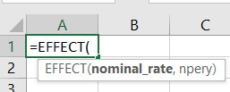
The function Effect is used to compute the yield.

Used factors / variable:

Information to input: (You can understand how to enter the Excel by seeing the picture below)

The yield for 7 per cent interest per annum is 7.19% when we receive interest once in three months.

Refer the table below to understand effect of getting monthly interest. It pushes the yield up by 7.23% per annum, even when the interest rate is only 7% per annum. 

Interest Frequency	Yield
Once in quarter	7.19
Once in half year	7.12
Once in month	7.23

In another example in Nov 19, popular NBFC is giving 7.72% interest – Interest distribution is every month, using the effect of 12 npery and rate of 7.72%, using effect function in excel we get 8% per annum interest.

Refer the image below for the same

Click the link to access the working model of the Payment template  in google sheets - You are free to change the variable and get the desired results. You can download and share with your contacts who are interested in this functions / learning excel 

Click here to read the NEXT article about using XIRR function: Mutual fund returns can be calculated using XIRR. The SBI Magnum multi-cab scheme is taken as an example and the period of investment is four years

Click here to read the PREVIOUS article about using FV function: Radha thinks he can buy a house in 10 years. Current price is  40  lakhs. Expected Inflation is 7%. Then how much money should he save now to buy a house in ten years?

Excel in Personal Finance - Part 2 - Function FV

Let us learn 5 Excel functions that are useful for personal finance

Click here to read: Introduction to Excel in Personal Finance
Click here to read: Excel Part 1 - Function PV

Function 2 - FV

FV - Calculating the required amount:

Radha thinks he can buy a house in 10 years. Current price is  40  lakhs. Expected Inflation is 7%. Then how much money should he save now to buy a house in ten years?

For this planning, before using Excel, we should better understand the factors/variables that have been used in the Excel function and correctly enter the numbers by input for those functions. The factors  used in the Excel distribution FV and in most of the financial functions, are given below

• "Rate" refers to rate of interest .
• "Nper" refers to the number of months / year in which the amount is paid in the SIP.
• The PMT is The amount of money we pay monthly.
• PV is the initial sum paid.
• FV is the amount available / received  at the end.
• "Type" is often taken as zero or one. (If the interest is paid upfront or at the end of the period)

To know the amount by FV: the interest rate is 7%, the period is ten years and the value is 40 lakhs.

Using FV function we are arriving the amount required after 10 years.

Used factors / variable:

Information to input:

If you submit the required inputs as shown above, the excel will calculate the FV. Here we get that the future price of the house is Rs 78,68,605 after 10 years.

You can understand how to enter the Excel role by looking at the following picture. In your computer, the cell number / reference may be different, but the input information must be exactly as shown in the picture with respect to variable as given in the problem.

Please click here to get the working model of this function in google sheet – you can try hands on using different variables suitable to your requirements.

Click here to read the NEXT article about using EFFECT function: Example: In the case of bank deposits, the Bank gives an annual interest of 7%. Here is the variation. One bank gives interest once a year. Another bank gives interest every six months but at the same 7% annual interest rate. If another bank gives interest once every three months, then we have to choose the bank who gives interest for a short period of time. This will give higher yield, which is slightly better than 7% per annum. Let us find how yield differs from bank to bank in the above example using excel effect function.

Click here to read the PREVIOUS article about using PV function : Karthik is planning to visit Europe in 5 years on estimated expense of 15 Lakhs. Read the article to find out how much he needs to invest now in lumpsum?

Excel in Personal Finance - Part 1 - Function PV

Let us learn 5 Excel functions that are useful for personal finance

Click here to read about Introduction to using excel / google sheet in finance

Function 1 - PV

PV - Calculating the required amount:

Karthik is planning to visit Europe in 5 year on estimated expense of 15 lakhs. How much he need to invest now in lumpsum?

For this planning, before using Excel, we should better understand the factors/variables that have been used in the Excel function and correctly enter the numbers by input for those functions. The factors  used in the Excel distribution FV and in most of the financial functions, are given below

• "Rate" refers to rate of interest .
• "Nper" refers to the number of months / year in which the amount is paid in the SIP.
• The PMT is The amount of money we pay monthly.
• PV is the initial sum paid.
• FV is the amount available / received  at the end.
• "Type" is often taken as zero or one. (If the interest is paid upfront or at the end of the period)

To know the present amount by PV: the interest rate is 10%, the period is 5  years and the value is 15 lakhs.

Using PV function we are arriving the amount required currently.

Used factors / variable:

Information to input:

If you submit the required inputs as shown above, the excel will calculate the PV. Here we get that the amount to be saved now for planned expenses is Rs 9,31,381.

You can understand how to enter the Excel role by looking at the following picture. In your computer, the cell number / reference may be different, but the input information must be exactly as shown in the picture with respect to variable as given in the problem.

Please click here to get the working model of this function in google sheet – you can try hands on using different variables suitable to your requirements.

Click here to read the NEXT article about using FV function: Radha thinks he can buy a house in 10 years. Current price is  40  lakhs. Expected Inflation is 7%. Then how much money should he save now to buy a house in ten years?